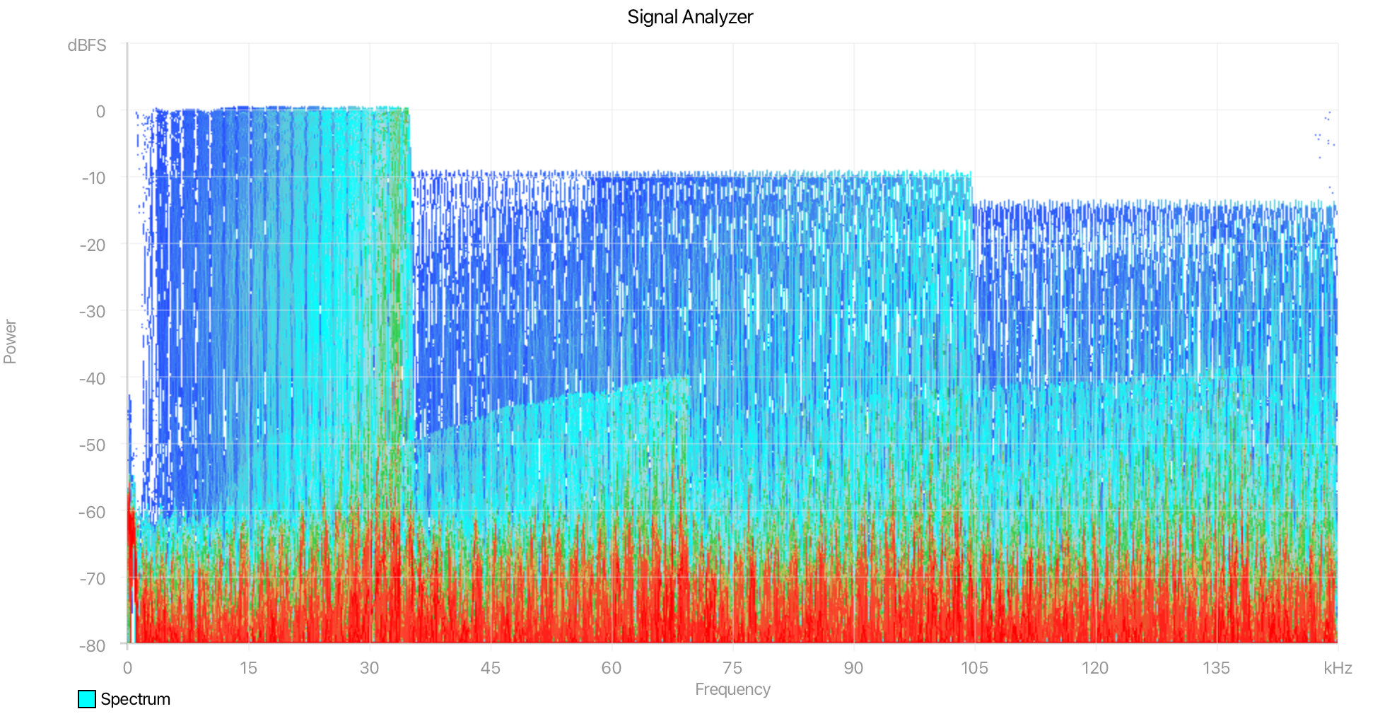
Controls
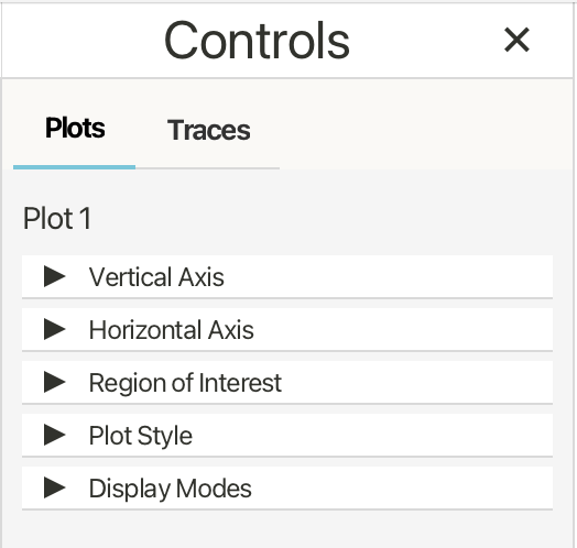
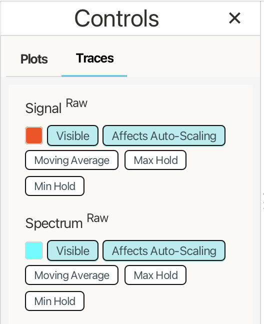
The Controls panel lets you view and edit plot and trace settings: axis ranges, titles, labels, trace colors, and more. You can enable display modes, add derived traces (moving average, max/min holds), hide traces, and edit trace colors. Everything that can be done with serial commands — and more — can be done directly within the Controls panel.
| Plots tab | Traces tab |
|---|---|
 |
 |
Selecting a Plot
![]()
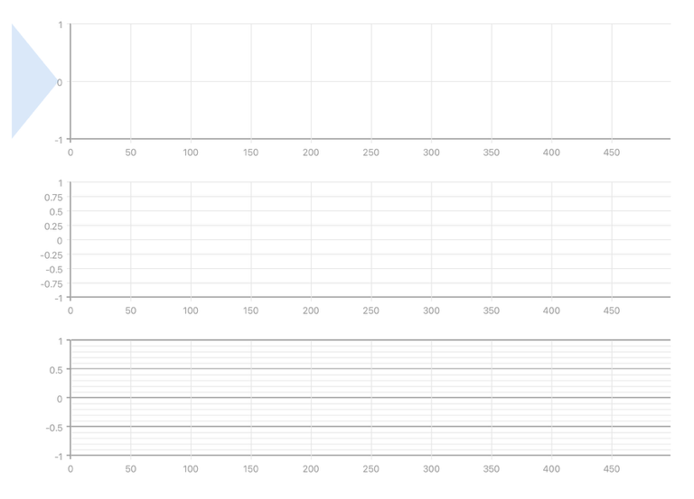
The Controls panel edits the currently selected plot. To select a plot, click inside the plot area. When more than one plot is visible, the selected plot is indicated by a subtle blue triangular marker along the left edge of the plot — like the illustration to the left of this paragraph.
You can also select plots with the keyboard using Ctrl+1 through Ctrl+8. The shortcut number is 1-based: Ctrl+1 selects the first (top) plot, Ctrl+2 selects the second plot down, and so on. If the requested plot number is higher than the number of visible plots, VoidLoop ViewPoint™ selects the last available plot.
Axis Configuration
The Axis sections control the scale, range, labels, units, and tick layout for the selected plot. Cartesian and scatter plots show Vertical Axis and Horizontal Axis sections. Polar plots show Radial Axis and Angular Axis sections.
Labels and Units
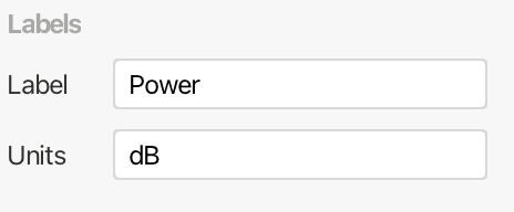
Cartesian and scatter axes can display a Label and Units. The label is the axis title shown beside or below the axis for the vertical and horizontal axis respectively. Units are short suffixes used in tick labels and readouts, such as V, Hz, or s. Each unit takes the place of the maximum tick value on the axis.
Scale
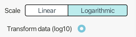
Axes that support logarithmic scaling can be set to Linear or Logarithmic. Logarithmic scale is available on Cartesian vertical axes, scatter horizontal and vertical axes, and polar radial axes. It is not available on Cartesian horizontal sample-index axes or polar angular axes.
When Logarithmic is selected, Transform data (log~10~) controls how values are handled. When enabled, VoidLoop ViewPoint™ applies a log~10~ transform to incoming values. When disabled, the data is treated as already logarithmic, and the axis bounds must remain positive.
Auto-Scale Strategies
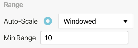
When Auto-Scale is enabled, the Scaling Strategy controls how VoidLoop ViewPoint™ chooses visible bounds over time. These strategies are available for auto-scaled linear data axes, except on Cartesian horizontal axes, which auto-increment by sample index.
Min Range sets the smallest span the axis is allowed to show while auto-scaling, defaulting to 10.
Windowed is the default method, scaling to the current data window with additional padding and clean tick intervals.
Expand Only grows the axis when new minimum or maximum values appear but does not shrink back automatically.
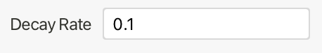
Peak Decay holds recent peaks and gradually relaxes back toward the current data range. The Decay Rate parameter controls how quickly the held bounds relax.
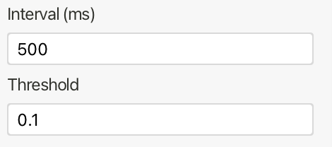
Debounced reduces visual jitter by limiting how often bounds update. Interval sets the minimum time between updates. Threshold sets the relative change required to force an immediate update.

Symmetric Zero keeps the axis symmetric around a center value. Center (default: 0) sets the midpoint of the visible range.
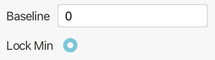
Baseline Zero locks one side of the axis to a baseline value and scales the other side. Baseline (default: 0) sets the anchor value. Lock Min keeps the minimum at the baseline; when Lock Min is off, the maximum is locked instead.

Robust Percentile ignores outliers by scaling to percentile bounds rather than absolute minimum and maximum. Low Percentile and High Percentile set the percentile range used for scaling.
Ticks
Ticks are available for manual, non-logarithmic axes.
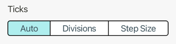
Auto enables derived tick spacing.
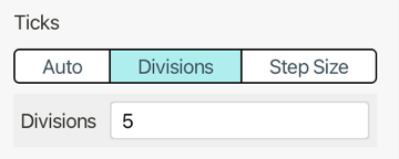
Divisions divides the visible range into a specified number of major intervals.
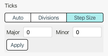
Step Size provides a way to specify major and minor tick spacing directly. Major ticks are labeled; minor ticks are drawn as smaller grid intervals and are not labeled.
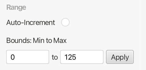
Bounds and Range
By default, an axis auto-scales to fit the incoming data. The Cartesian horizontal axis auto-increments with the sample index. When Auto-Scale or Auto-Increment is disabled, Bounds: Min to Max sets the fixed visible range for the axis. The minimum must be less than the maximum.
| Manual bounds | Auto-increment |
|---|---|
 |
 |
Horizontal Axis: Auto-Increment
For Cartesian plots, the horizontal axis represents the sample index. When Auto-Increment is enabled, the horizontal axis advances automatically from the first sample in the current data window to the last sample.
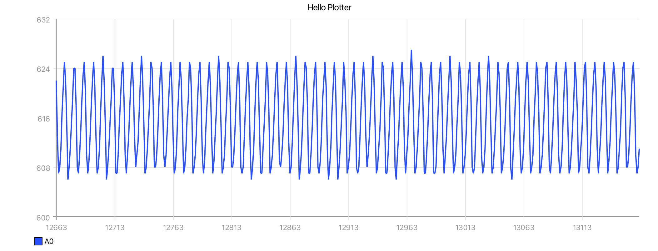
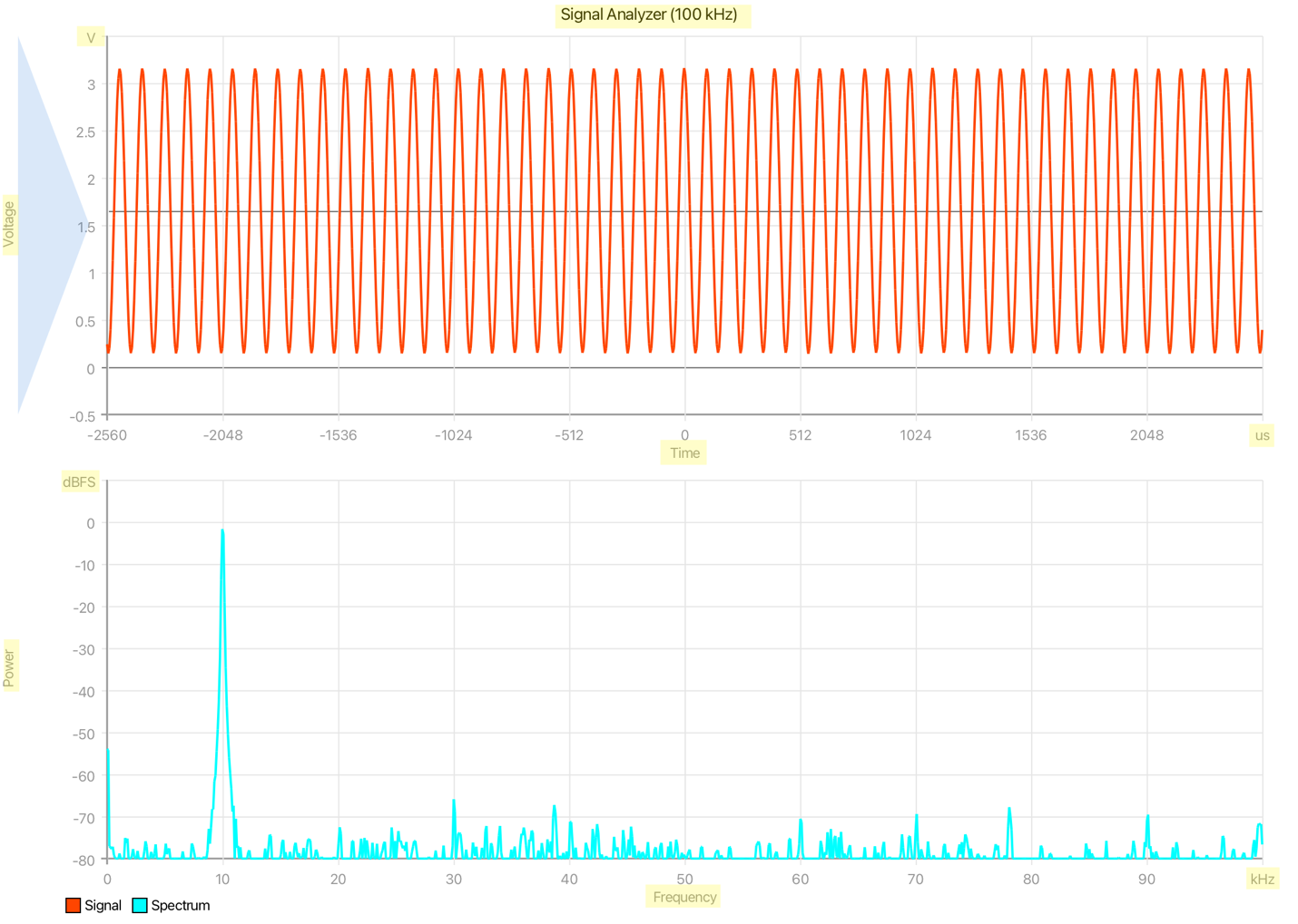
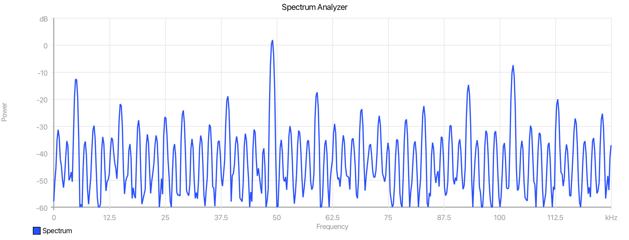
Horizontal Axis: Domain Labels
There are use cases where the horizontal axis represents a domain other than the sample index, like the frequency domain. This can be achieved by setting the axis range for the horizontal axis. This action disables Auto-Increment and adjusts the horizontal axis labeling, not the actual bounds — by default the same set of data is in view, only the tick labels are adjusted.
The vertical axis uses Auto-Scale to fit the incoming trace data. Additional information is available on the various auto-scaling techniques under Auto-Scale Strategies.
For scatter plots, both horizontal and vertical axes represent data values. When Auto-Scale is enabled, each axis can scale to the data assigned to that axis.
Polar Properties
Polar plots use a Radial Axis and an Angular Axis. The Radial Axis behaves like a value axis and supports auto-scale, scaling strategies, manual bounds, ticks, and logarithmic scale.
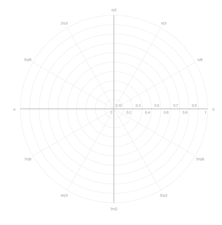
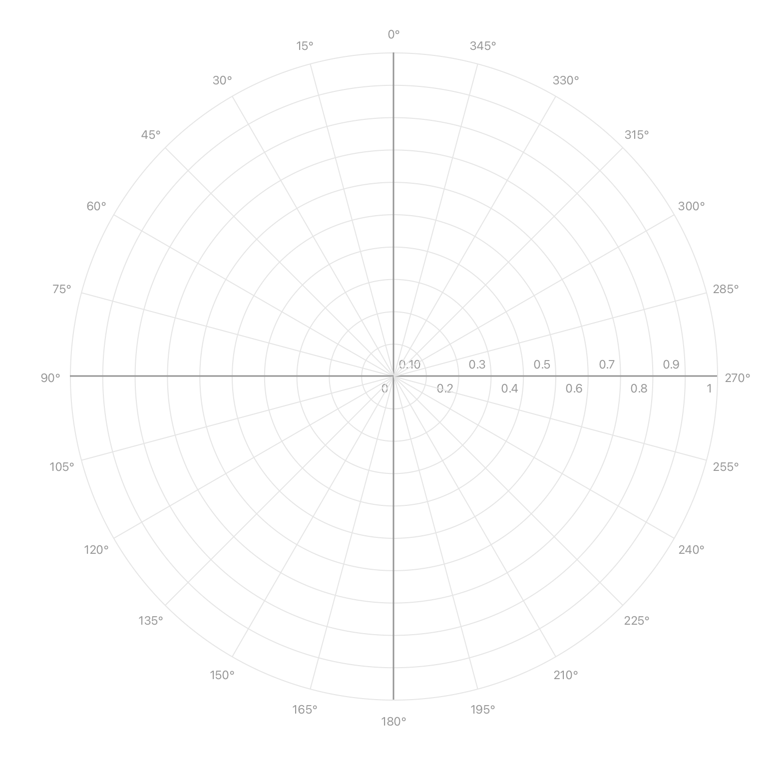
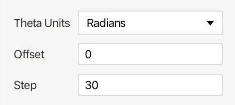
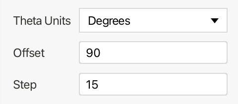
The Angular Axis controls theta. Theta Units switches the angular display between Degrees and Radians. Offset rotates the angular axis by the specified amount. Step sets the angular spacing between major divisions.
| Radians | Degrees |
|---|---|
 |
 |
 |
 |
Polar plots do not expose Cartesian-style axis labels or units in the Controls panel.
Frame Decay (Scatter and Polar plots)
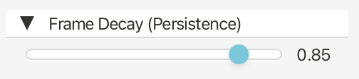
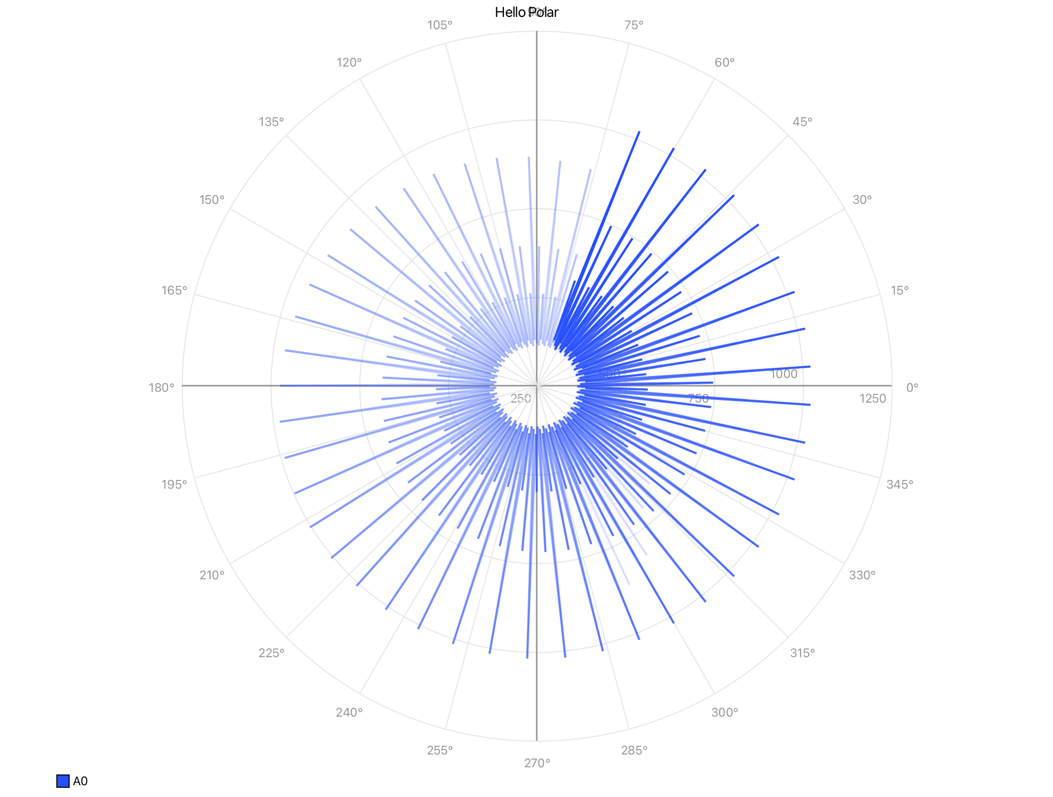
Frame Decay applies a per-sample alpha gradient across the points within a single frame, mapping sample age to opacity: the most recently received sample is drawn fully opaque, and each preceding sample is attenuated by a decay factor. The decay value sets the length of this gradient — higher values extend the visible trail by fading older samples more slowly, while lower values collapse the frame down to only the newest points.
This matters because scatter and polar traces are not single-valued along a monotonic axis. Unlike a time-domain line plot, where each x maps to one y and ordering is implicit in position, a scatter or polar trace can revisit the same region, wind through multiple revolutions, or cross over itself within one frame. Spatial position alone therefore carries no information about sample order. Frame Decay restores that ordering by encoding it as an opacity ramp, so the eye can recover direction of travel and distinguish leading edge from trailing history even where the geometry overlaps.
Frame Decay is distinct from the Persistence display mode, and the two operate at different scopes:
- Frame Decay acts within a single frame, in both Continuous and Frames update modes, fading samples relative to one another based on their order of arrival. It governs intra-frame point opacity only.
- Persistence acts across frames, in Frames mode only, compositing previously rendered frames beneath the current one to show evolution over time.
Region of Interest
The Region of Interest section lets you zoom into part of a Cartesian or scatter plot.
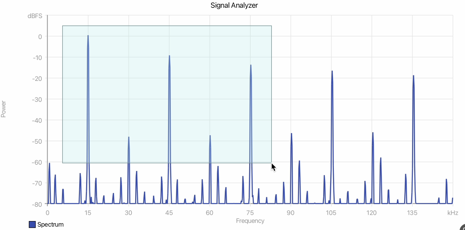
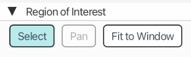
Select enables ROI selection mode. With selection mode active, click and drag inside the plot to choose a region. Releasing the mouse zooms the plot to that region. Press Z to toggle selection mode from the keyboard.
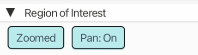
Pan is available after the plot is zoomed. When Pan is enabled, drag inside the plot to move the zoomed region. Press P to toggle Pan, or right-click and drag to pan temporarily.
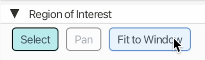
Fit to Window restores the full plot bounds and keeps ROI selection active. Double-clicking inside the plot performs the same fit-to-window action. Press F while ROI mode is active to fit to window. Press Esc to exit ROI mode.
Note
These keyboard shortcuts are case-insensitive — Shift-Z and z both activate
zoom, Shift-P and p both activate panning, and so on.
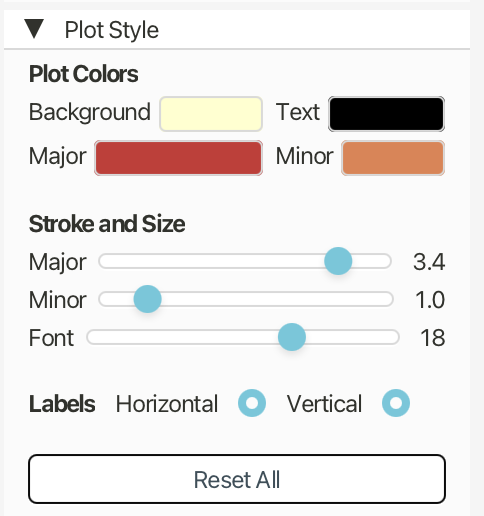
Plot Style
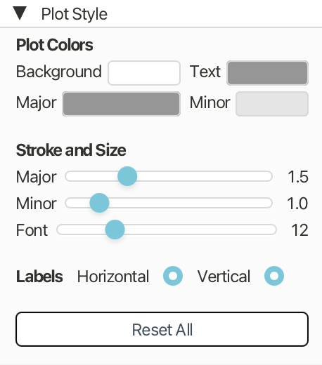
Plot Style controls visual styling for the selected plot.
Plot Colors sets the plot background, axis and tick text color, major grid line color, and minor grid line color.
Stroke and Size set the major grid line thickness, minor grid line thickness, and axis/tick label font size.
Labels controls whether horizontal and vertical axis labels are shown.
Reset All clears plot-specific style overrides and returns the plot to the default style.
| Custom colors | Result |
|---|---|
 |
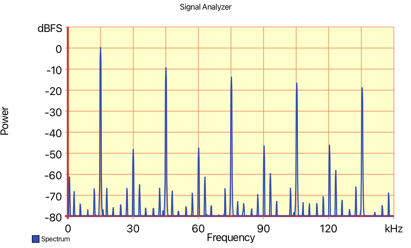 |
Display Modes

Display Modes are available for non-polar plots when the plotter is in the Frames update mode. Only one display mode per plot can be active at a time.
Grid Opacity controls how visible the grid lines are while a display mode is active. Enabling a display mode usually lowers grid opacity so the rendered history is easier to see.
Persistence
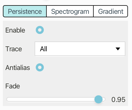
Persistence overlays recent frames to show signal persistence over time.
Enable turns the mode on or off.
Trace selects which trace contributes to the persistence image, or All for all traces.
Antialias smooths persistence line edges.
Fade controls how quickly older persistence frames disappear; lower values fade faster, while higher values retain history longer.
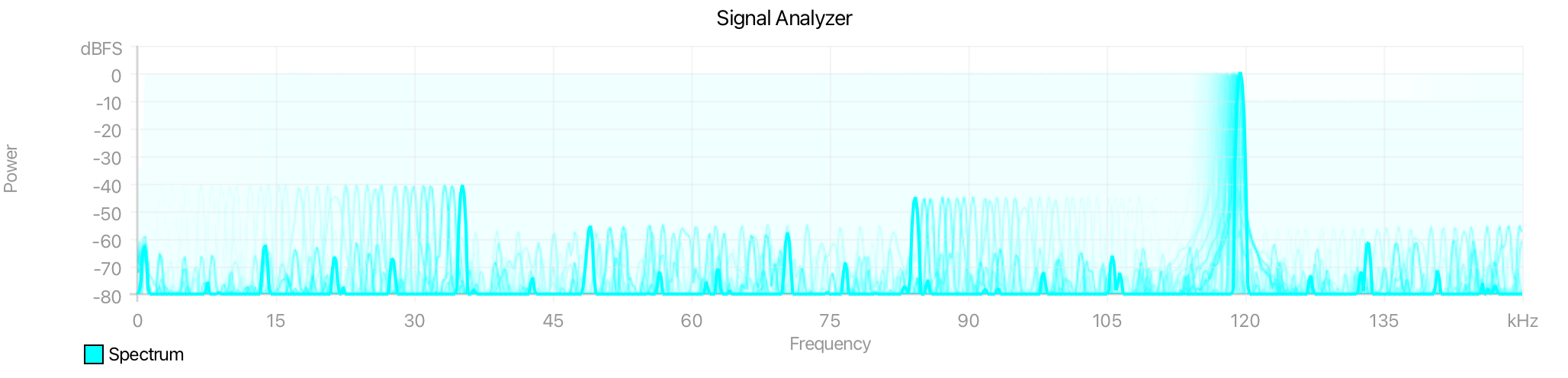
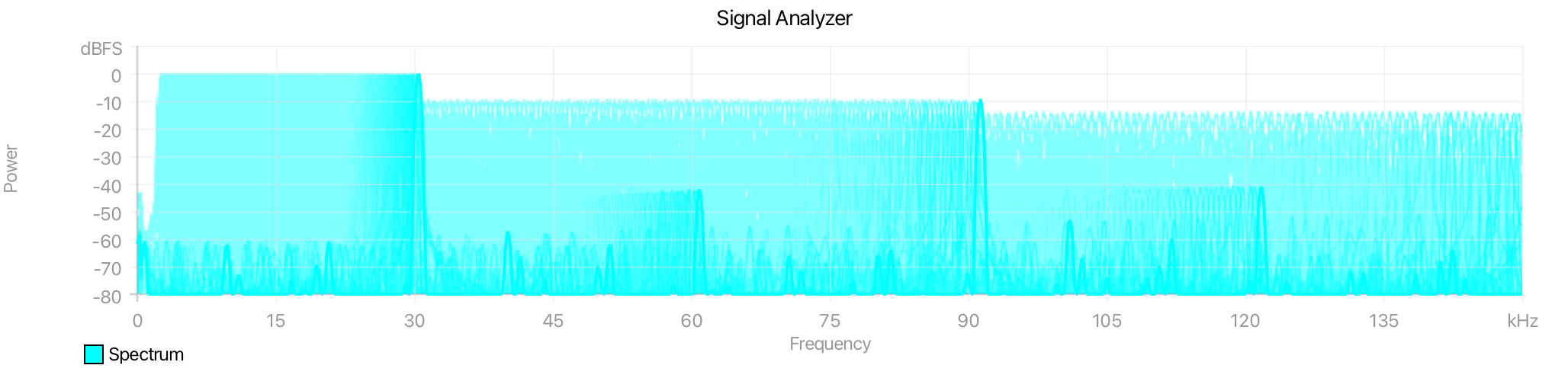
Spectrogram
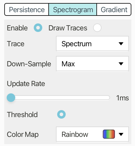
Spectrogram renders incoming data as a time-history image where amplitude is mapped to color.
Enable turns the mode on or off.
Draw Traces overlays normal trace lines on top of the spectrogram.
Trace selects the source trace.
Down-Sample chooses how each time bucket is reduced: Max preserves peaks, while Average smooths values.
Update Rate sets the time bucket size.
Threshold clamps values below the amplitude floor to black.
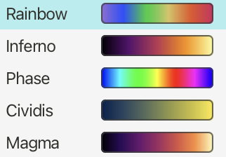
Color Map selects the color gradient.

Gradient
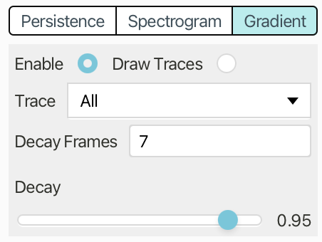
Gradient accumulates hit counts per pixel and maps frequency to color.
Enable turns the mode on or off.
Draw Traces overlays normal trace lines on top of the gradient image.
Trace selects the source trace, or All.
Decay Frames sets how often accumulated hit counts decay.
Decay sets the per-frame fade factor; lower values fade older data faster.