Concepts

This page explains the ideas you need to use SignalCore well: how the library is put together, how a spectrum is laid out and read, how windowing and the DC bin shape a measurement, and what the signal generator and streaming processors are for. Each section names the calls involved. The API Reference has the full signatures, and the Recipes put these ideas to work on specific jobs.

The signalcore namespace

Every type and function in the library lives in a namespace called signalcore. A namespace is a named scope. Because SignalCore uses short, common words like FFT, Trigger, and Sine, the namespace keeps those identifiers from colliding with names in your own sketch or in another library.

The usual pattern is to bring the namespace into scope once, right after the include:

#include <SignalCore.h>
using namespace signalcore;

With that using line in place you write FFT<1024>, SignalGenerator, and WindowType::BlackmanHarris directly. Leave it out and you spell each name with the signalcore:: prefix instead (signalcore::FFT<...>). That is worth doing only if one of these names happens to clash with something else in your sketch.

How the library is organized

SignalCore is header-only: there is no separate library file to compile or link against. Including a header copies its code into your sketch when it builds, so installing the library is just a matter of making the headers available to the compiler. There is no build step to set up.

SignalCore.h is an umbrella header that includes every module at once. It is the simplest way to start, and what the examples use:

Module	Header	What it's for
FFT	signalcore/FFT.h	Frequency analysis: the FFT<> transform plus peak-finding and signal-quality metrics
DDS	signalcore/DDS.h	Generating signals in software: the high-level SignalGenerator and the lower-level DDS oscillator
Windows	signalcore/Windows.h	Window functions that reduce spectral leakage before a transform
Trigger	signalcore/Trigger.h	Edge triggering to hold a repeating waveform still, oscilloscope-style
PeakHold	signalcore/PeakHold.h	Per-bin max-hold for spectrum displays
MovingAverage	signalcore/MovingAverage.h	Exponential smoothing of a spectrum or signal
Platform	signalcore/Platform.h	Board and backend detection, plus math helpers the other modules rely on

Including SignalCore.h pulls in all of it. If a sketch needs only one or two modules and program memory (flash) is tight on a small board, include just those headers instead. For example, #include <signalcore/FFT.h> pulls in only the FFT module for a spectrum-only sketch, and the compiler leaves the rest out.

The same results on every board

A fair question for any cross-platform library is whether an FFT will give the same answer on a Teensy as on an ESP32. SignalCore is built so that it does.

The FFT has two interchangeable implementations, and the library selects one for you when the sketch compiles:

Implementation	When it is used
CMSIS-DSP (hardware-accelerated)	On Teensy 4.x, automatically. CMSIS-DSP is ARM's optimized signal-processing library; on a Teensy it runs the transform much faster than plain C++ can.
Portable C++	On every other board: a self-contained power-of-two FFT that needs no special hardware or extra libraries (radix-2 Cooley-Tukey implementation).

The selection is conservative on purpose. Some ARM cores ship the CMSIS headers but do not actually link the compiled DSP code, which would make a build fail at the last step. To avoid that, automatic use is limited to Teensy 4.x, where the toolchain is known to provide the whole library. Other ARM boards (Arduino Giga, STM32, SAMD51) can opt in with a single define before the include:

#define SIGNALCORE_FORCE_CMSIS
#include <SignalCore.h>

See Configuration & Platforms for more.

The key point is that both implementations produce the same spectrum, bin for bin. You can develop a spectrum-analysis sketch on a Teensy and deploy it on an ESP32, or the reverse, without changing any of the spectral code.

How data flows

Almost every SignalCore sketch follows one of two paths, and both begin with a buffer of samples. Those samples can come from real hardware, such as analogRead() on an ADC pin, or from the built-in SignalGenerator when you have no signal source on hand.

The first path is frequency analysis. You hand a block of samples to fft.calculate(), which windows them, runs the transform, and leaves a magnitude spectrum in its result buffer. From there you read numbers off the spectrum. peakBin() and peakFrequency() give the strongest frequency, SINAD() and ENOB() grade the signal's quality, and passing the spectrum through ExponentialMovingAverage or PeakHoldProcessor steadies it for a display. When you want the values in decibels, postScaleDB() converts the buffer in place.

The second path stays in the time domain. Instead of building a spectrum, it finds a stable starting point in the samples so a repeating waveform stops scrolling across the display. You capture into a buffer larger than the frame you intend to draw, and trig.calculateOffset() returns a pointer into that buffer, positioned so a chosen edge sits at a fixed place in the frame. An edge here is simply the moment the signal crosses a threshold level. This is the same idea as the trigger control on an oscilloscope.

A scope-style sketch often runs both paths over a single capture buffer, so the same data appears at once as a spectrum and as a steady, triggered trace. The Recipes build each path step by step. For a detailed example of both paths, that streams data to ViewPoint to be visualized see the ViewPoint example Cartesian/SignalAnalyzer_A0.

Window functions

When an FFT runs on a chunk of samples, it treats that chunk as if it repeats forever. If the signal does not complete a whole number of cycles in the chunk, the two ends do not line up, and the transform smears the tone's energy across neighboring bins. That smearing is called spectral leakage, and it can bury a small tone sitting next to a large one.

A window reduces leakage by tapering the samples toward zero at both ends before the transform, so the chunk joins smoothly to its imagined neighbor. The cost is that tapering slightly widens the main peak. Each window strikes that balance between a narrow peak and low leakage differently.

SignalCore ships ten windows as the WindowType enum: Rectangle, Hamming, Hann, Triangle (also called Bartlett), Nuttall, Blackman, BlackmanNuttall, BlackmanHarris, FlatTop, and Welch. None is also accepted and means no taper at all, the same as Rectangle. Set a window once on the FFT object:

fft.setWindowType(WindowType::BlackmanHarris);

To save RAM, the FFT keeps only the first half of a window's coefficients and mirrors them across the center, since every window it ships is symmetric. The Rectangle and None windows apply no taper, so they skip the multiply step entirely. The Recipes include a table of which window to reach for and an example that measures the leakage difference between them.

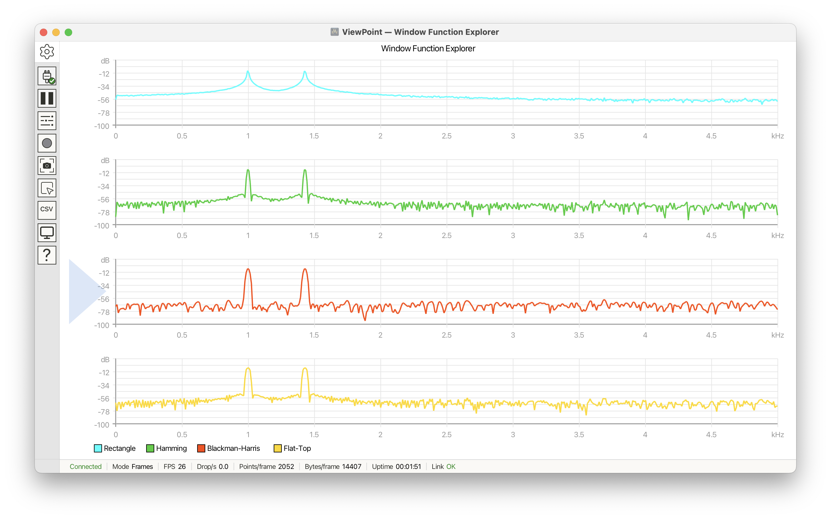
ViewPoint contains an example, Cartesian/WindowFunctionExplorer that helps visualize the effect of different windows on the same data.

FFT output format

A real-input FFT of N samples produces N/2 + 1 useful values, called bins. Each bin holds the magnitude, the strength, of one frequency. The rest of the transform's output is a mirror image of these bins and carries no new information, so SignalCore leaves the useful bins in the result buffer and you ignore the rest.

Index	Contents
result[0]	DC, the average level of the signal
result[1 .. N/2 - 1]	Magnitude of each frequency between DC and Nyquist
result[N/2]	Nyquist, the highest frequency the FFT can represent (half the sample rate)

You read the spectrum straight off the FFT object. It converts to a float*, so you can treat it like a plain array of magnitudes:

float* spectrum = (float*)fft;
float  thirdBin = spectrum[3];

The internal layout before this point, where real and imaginary parts sit interleaved in the same array, is described in the API Reference. You do not need it to read a result.

The DC bin

Bin 0 is the one to watch when you are looking for a tone. Any constant offset in the input, called DC, lands entirely in bin 0. On raw ADC data that offset is often taller than the signal itself, so a naive search for the tallest bin would return bin 0 every time.

Two habits keep DC out of the way. The first is to remove it before the transform with removeDC(), which flattens bin 0 to almost nothing. The second is to start the peak search at bin 1 instead of bin 0. findPeak takes a start index for exactly this, and it returns an absolute bin number, so there is nothing to adjust afterward:

float* spectrum = (float*)fft;
int    peakBin  = findPeak(spectrum, N / 2 + 1, /*start=*/1);   // skip DC

For the common case the FFT does this bookkeeping for you. fft.peakBin() returns the dominant bin with DC already skipped, and fft.peakFrequency(sampleRate) gives that frequency in Hz.

removeDC() is the real fix. Starting at bin 1 is the backstop for the integer path, where calculate(uint16_t*) reads ADC counts directly and cannot subtract the bias for you. Once you have read the linear magnitudes, convert them to decibels in place with postScaleDB(). If log10f is too heavy on a slower board, postScaleDBFast() trades a little accuracy for speed.

Signal generation

Sometimes you need a signal and have no hardware to read, or you want a known, clean input to test your processing against. SignalCore can synthesize one in software, at two levels of control.

SignalGenerator is the high-level path and the one most sketches use. You set a carrier shape and frequency, optionally add amplitude modulation and gaussian noise, then pull samples one at a time with nextSample(). It is well suited to feeding synthetic data into an FFT while you develop a spectrum sketch.

SignalGenerator sig(SAMPLE_RATE);
sig.setCarrier(SignalShape::Sine, 1000.0);   // 1 kHz sine
float s = (float)sig.nextSample(0);          // 0 means full-resolution float

DDS together with DDSSineTable<> is the low-level path. It is a phase-accumulator oscillator: a 32-bit counter advances by a fixed step each sample and indexes a pre-built wave table, which is an efficient way to produce a steady tone. DDSSineTable<> fills that table when it is constructed and keeps it in RAM — 4 bytes per sample (Samples1024 = 4 KB), so size the table to your board. Reach for this when you want tight, table-driven tone generation and do not need modulation or noise.

SignalShape selects the waveform for both the carrier and the modulation source. The choices are Sine, Square, Triangle, Sawtooth, Noise, and None.

Streaming processors

Three classes work on a running stream of data across many calls, rather than on a single one-shot buffer. PeakHoldProcessor and ExponentialMovingAverage keep their results in an internal array that you read back the same way as an FFT result, either by indexing it or by reading it as a float*. Trigger owns no result array: calculateOffset() returns a pointer into the capture buffer you pass it, and valid() says whether that pointer is edge-aligned.

Trigger finds a rising or falling edge in a sample buffer and reports an offset so that edge sits at a fixed position in the frame you draw. It uses hysteresis, a small margin around the threshold, so that noise wobbling across the threshold does not fire a burst of false triggers. This is the standard way to hold an oscilloscope-style trace still.

PeakHoldProcessor keeps a running maximum for each element and lets each held peak fade slowly back toward the live value. A decay factor controls the fade, and a value closer to 1.0 holds the peaks longer. It is common for the max-hold bars on a spectrum analyzer and for envelope following.

ExponentialMovingAverage smooths each element over time. It is a single-pole filter, meaning each output is a blend of the newest sample and the previous output, weighted by sampleWeight (the smoothing factor DSP texts often call alpha). A smaller sampleWeight smooths harder and responds more slowly. Note that sampleWeight and decay are opposite conventions, so do not copy one value into the other.

PeakHoldProcessor and ExponentialMovingAverage allocate their internal arrays when constructed. On a RAM-tight board such as an AVR, create them once at the size you need early in setup(), rather than resizing them repeatedly in the loop. That keeps the heap from fragmenting.

---

Created by VoidLoop · Founded by Gregory Kovacs · Written by Zachariah Magee